Forward computation

Recall, to compute source estimates, one typically assumes:

$M = GX + E$

where $M \in \mathbb{R}^{C \times T}$ is the sensor data, $G \in \mathbb{R}^{C \times S}$ is the lead-field matrix, $X \in \mathbb{R}^{S \times T}$ is the source time course (stc) and $E \in \mathbb{R}^{C \times T}$ is additive Gaussian noise

The lead-field matrix or forward operator $G$ is computed using the physics of the problem. It is what we will focus on here

import matplotlib.pyplot as plt

from IPython.display import Image
from mayavi import mlab
mlab.init_notebook('png')

Notebook initialized with png backend.

Computing the forward operator

To compute a forward operator we need:

the BEM surfaces
a -trans.fif file that contains the coregistration info
a source space

import mne
from mne.datasets import sample

data_path = sample.data_path()

# the raw file containing the channel location + types
raw_fname = data_path + '/MEG/sample/sample_audvis_raw.fif'

# The transformation file obtained by coregistration
trans = data_path + '/MEG/sample/sample_audvis_raw-trans.fif'
# The paths to freesurfer reconstructions
subjects_dir = data_path + '/subjects'

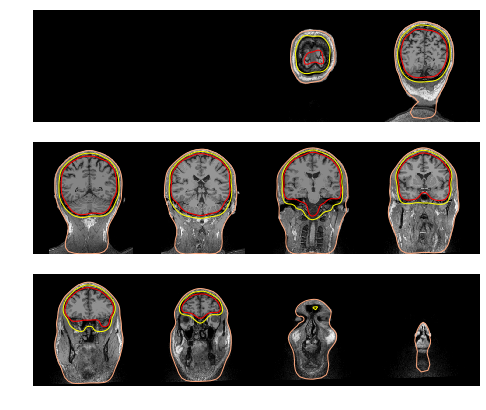
Compute and visualize BEM surfaces

Computing the BEM surfaces requires FreeSurfer and makes use of either of the two following command line tools:

Here we’ll assume it’s already computed. It takes a few minutes per subject.

So first look at the BEM surfaces.

For EEG we use 3 layers (inner skull, outer skull, and skin) while for MEG 1 layer (inner skull) is enough.

%matplotlib inline
mne.viz.plot_bem(subject='sample', subjects_dir=subjects_dir,
                 orientation='coronal');

Using surface: /home/mainak/Desktop/projects/github_repos/mne-python/examples/MNE-sample-data/subjects/sample/bem/inner_skull.surf
Using surface: /home/mainak/Desktop/projects/github_repos/mne-python/examples/MNE-sample-data/subjects/sample/bem/outer_skull.surf
Using surface: /home/mainak/Desktop/projects/github_repos/mne-python/examples/MNE-sample-data/subjects/sample/bem/outer_skin.surf

png

conductivity = (0.3,)  # for single layer
# conductivity = (0.3, 0.006, 0.3)  # for three layers
model = mne.make_bem_model(subject='sample', ico=4,
                           conductivity=conductivity,
                           subjects_dir=subjects_dir)
bem = mne.make_bem_solution(model)

Creating the BEM geometry...
Going from 4th to 4th subdivision of an icosahedron (n_tri: 5120 -> 5120)
inner skull CM is   0.67 -10.01  44.26 mm
Surfaces passed the basic topology checks.
Complete.

Approximation method : Linear collocation

Homogeneous model surface loaded.
Computing the linear collocation solution...
    Matrix coefficients...
        inner skull (2562) -> inner skull (2562) ...
    Inverting the coefficient matrix...
Solution ready.
BEM geometry computations complete.

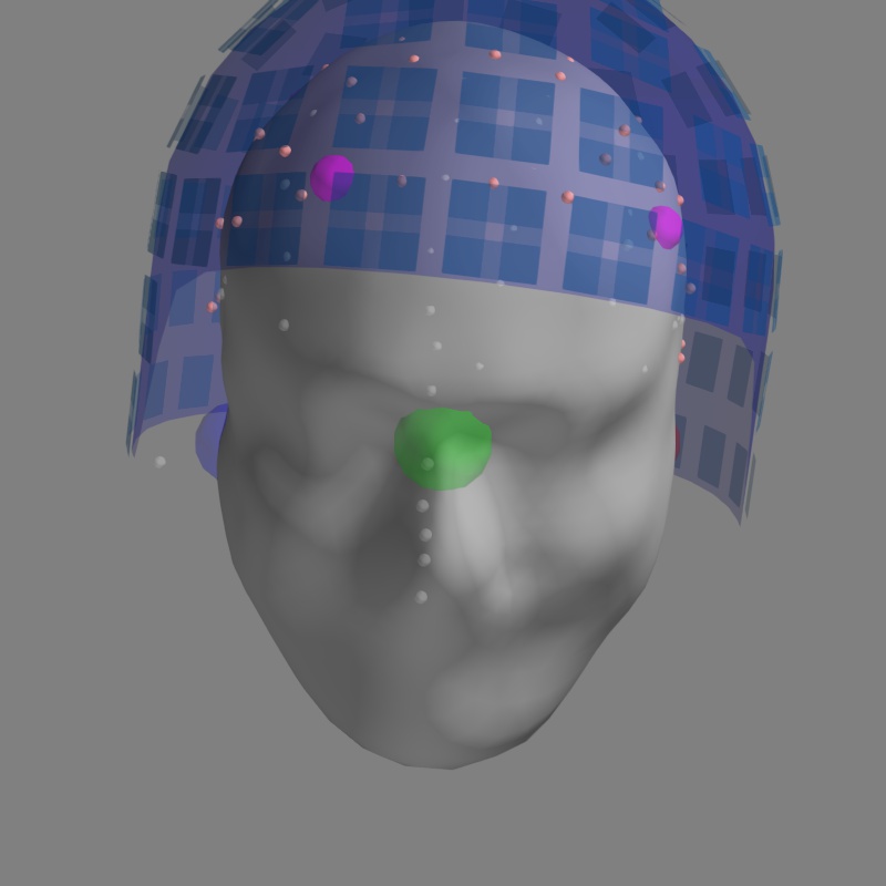
Visualization the coregistration

The coregistration is operation that allows to position the head and the sensors in a common coordinate system. In the MNE software the transformation to align the head and the sensors is stored in a so called trans file. It is a FIF file that ends with -trans.fif.

It can be obtained with

mne_analyze (Unix tools)
mne.gui.coregistration (in Python), or
mrilab if you’re using a Neuromag system.

For the Python version see http://martinos.org/mne/dev/generated/mne.gui.coregistration.html

Here we assume the coregistration is done, so we just visually check the alignment with the following code.

info = mne.io.read_info(raw_fname)
fig = mne.viz.plot_alignment(info, trans, subject='sample', dig=True,
                             subjects_dir=subjects_dir, verbose=True);
mlab.savefig('coreg.jpg')
Image(filename='coreg.jpg', width=500)

    Read a total of 3 projection items:
        PCA-v1 (1 x 102)  idle
        PCA-v2 (1 x 102)  idle
        PCA-v3 (1 x 102)  idle
Using outer_skin.surf for head surface.
Getting helmet for system 306m

jpeg

mlab.close()

Compute Source Space

The source space defines the position of the candidate source locations.

The following code compute such a source space with an OCT-6 resolution.

mne.set_log_level('WARNING')
subject = 'sample'
src = mne.setup_source_space(subject, spacing='oct6',
                             subjects_dir=subjects_dir,
                             add_dist=False)

src

<SourceSpaces: [<surface (lh), n_vertices=155407, n_used=4098, coordinate_frame=MRI (surface RAS)>, <surface (rh), n_vertices=156866, n_used=4098, coordinate_frame=MRI (surface RAS)>]>

src contains two parts, one for the left hemisphere (4098 locations) and one for the right hemisphere (4098 locations).

Let’s write a few lines of mayavi to see what it contains

import numpy as np
from surfer import Brain

brain = Brain('sample', 'lh', 'white', subjects_dir=subjects_dir)
surf = brain.geo['lh']

vertidx = np.where(src[0]['inuse'])[0]

mlab.points3d(surf.x[vertidx], surf.y[vertidx],
              surf.z[vertidx], color=(1, 1, 0), scale_factor=1.5)

mlab.savefig('source_space_subsampling.jpg')
Image(filename='source_space_subsampling.jpg', width=500)

jpeg

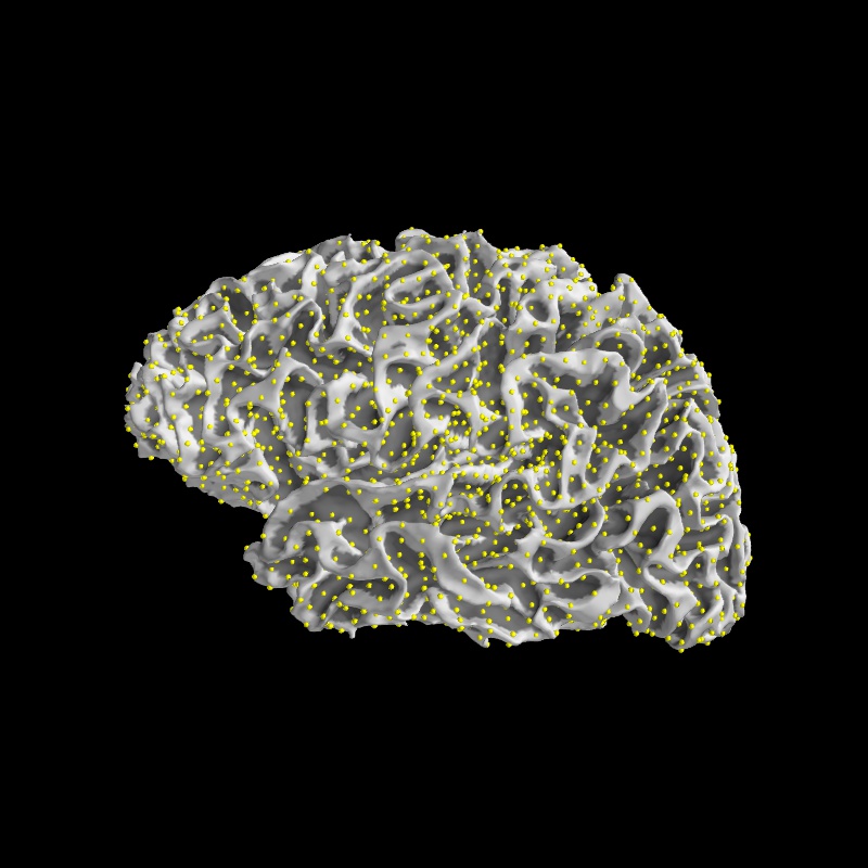
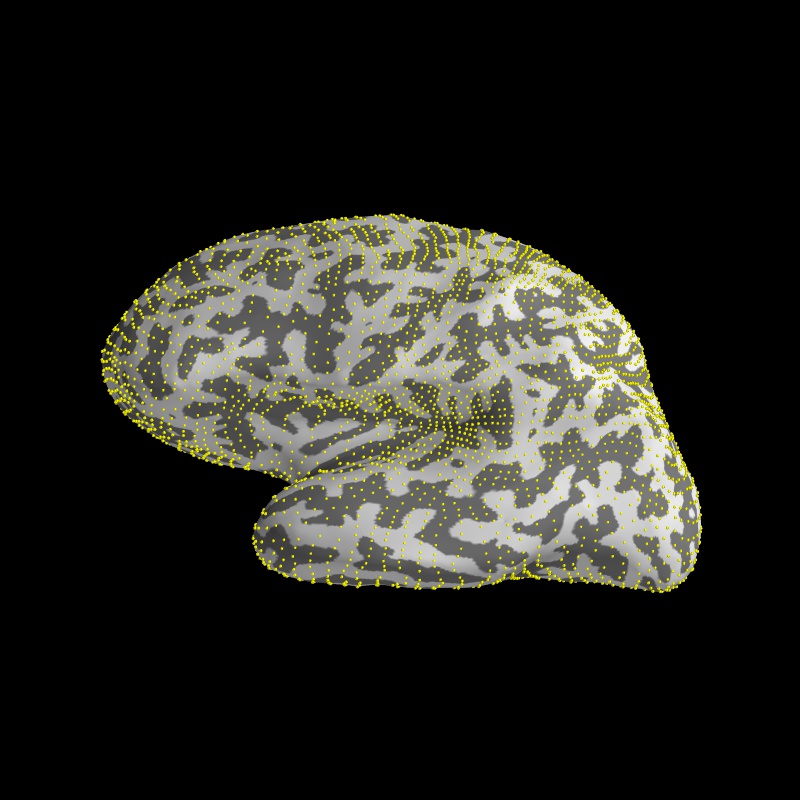
Since it’s hard to see the source points on the walls of the sulcus, it is common practice to inflate the white matter surface

brain = Brain('sample', 'lh', 'inflated', subjects_dir=subjects_dir)
surf = brain.geo['lh']

mlab.points3d(surf.x[vertidx], surf.y[vertidx],
              surf.z[vertidx], color=(1, 1, 0), scale_factor=1.5)

mlab.savefig('source_space_subsampling.jpg')
Image(filename='source_space_subsampling.jpg', width=500)

jpeg

mlab.close()

Compute forward solution

We can now compute the forward solution.

To reduce computation we’ll just compute a single layer BEM (just inner skull) that can then be used for MEG (not EEG).

# Name of the forward to read (precomputed) or compute
fwd_fname = data_path + '/MEG/sample/sample_audvis-meg-eeg-oct-6-fwd.fif'
fwd = mne.make_forward_solution(raw_fname, trans=trans, src=src, bem=bem,
                                meg=True, # include MEG channels
                                eeg=False, # include EEG channels
                                mindist=5.0, # ignore sources <= 5mm from inner skull
                                n_jobs=1) # number of jobs to run in parallel

fwd

<Forward | MEG channels: 306 | EEG channels: 0 | Source space: Surface with 7498 vertices | Source orientation: Free>

Or read the EEG/MEG file from disk

fwd = mne.read_forward_solution(fwd_fname)

fwd

<Forward | MEG channels: 306 | EEG channels: 60 | Source space: Surface with 7498 vertices | Source orientation: Free>

Convert to surface orientation for cortically constrained inverse modeling

fwd = mne.convert_forward_solution(fwd, surf_ori=True)
leadfield = fwd['sol']['data']
print("Leadfield size : %d sensors x %d dipoles" % leadfield.shape)

Leadfield size : 366 sensors x 22494 dipoles

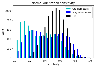
Sensitivy maps

Recall we had the gain matrix $G \in \mathbb{R}^{S \times C}$.

A column in this matrix $g \in \mathbb{R}^{C}$ tells us how much each sensor is to a particular source

We can compute the sensitivity $a_s$ of the signals to each source point as:

$a_s = \sqrt(g^{\top}g)$

grad_map = mne.sensitivity_map(fwd, ch_type='grad', mode='fixed')
mag_map = mne.sensitivity_map(fwd, ch_type='mag', mode='fixed')
eeg_map = mne.sensitivity_map(fwd, ch_type='eeg', mode='fixed')

%matplotlib inline
plt.hist([grad_map.data.ravel(), mag_map.data.ravel(), eeg_map.data.ravel()],
          bins=20, label=['Gradiometers', 'Magnetometers', 'EEG'],
         color=['c', 'b', 'k'])
plt.legend()
plt.title('Normal orientation sensitivity')
plt.xlabel('sensitivity')
plt.ylabel('count');

png

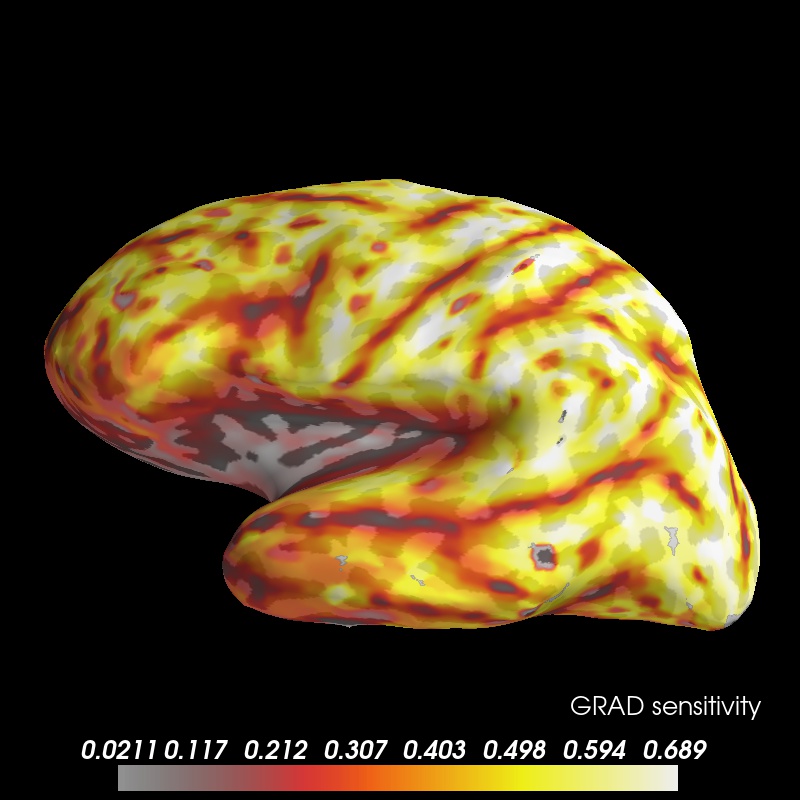
clim = dict(kind='percent', lims=(0.0, 50, 95), smoothing_steps=3)  # let's see single dipoles
brain = grad_map.plot(subject='sample', time_label='GRAD sensitivity', surface='inflated',
                      subjects_dir=subjects_dir, clim=clim, smoothing_steps=8, alpha=0.85);
view = 'lat'
brain.show_view(view)
brain.save_image('sensitivity_map_grad_%s.jpg' % view)
Image(filename='sensitivity_map_grad_%s.jpg' % view, width=400)

jpeg

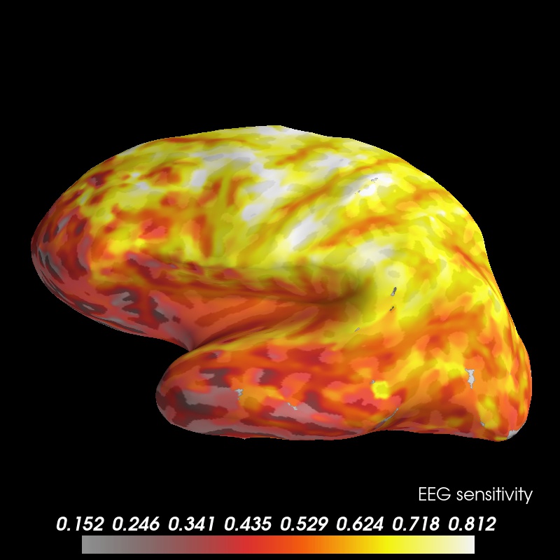
clim = dict(kind='percent', lims=(0.0, 50, 99), smoothing_steps=3)  # let's see single dipoles
brain = eeg_map.plot(subject='sample', time_label='EEG sensitivity', surface='inflated',
                     subjects_dir=subjects_dir, clim=clim, smoothing_steps=8, alpha=0.9);
view = 'lat'
brain.show_view(view)
brain.save_image('sensitivity_map_eeg_%s.jpg' % view)
Image(filename='sensitivity_map_eeg_%s.jpg' % view, width=400)

jpeg

mlab.close()

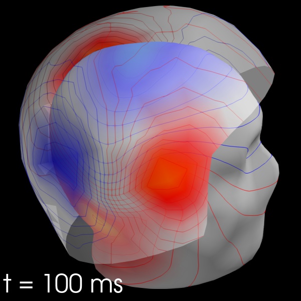
Visualizing field lines based on coregistration

from mne import read_evokeds
from mne.datasets import sample
from mne import make_field_map

data_path = sample.data_path()

raw_fname = data_path + '/MEG/sample/sample_audvis_filt-0-40_raw.fif'

subjects_dir = data_path + '/subjects'
evoked_fname = data_path + '/MEG/sample/sample_audvis-ave.fif'
trans_fname = data_path + '/MEG/sample/sample_audvis_raw-trans.fif'

make_field_map?

# If trans_fname is set to None then only MEG estimates can be visualized

condition = 'Left Auditory'
evoked_fname = data_path + '/MEG/sample/sample_audvis-ave.fif'
evoked = mne.read_evokeds(evoked_fname, condition=condition, baseline=(-0.2, 0.0))

# Compute the field maps to project MEG and EEG data to MEG helmet
# and scalp surface
maps = mne.make_field_map(evoked, trans=trans, subject='sample',
                      subjects_dir=subjects_dir, n_jobs=1)

# explore several points in time
field_map = evoked.plot_field(maps, time=.1);

from mayavi import mlab
mlab.savefig('field_map.jpg')
from IPython.display import Image
Image(filename='field_map.jpg', width=800)

jpeg

mlab.close()

Exercise

Plot the sensitivity maps for EEG and compare it with the MEG, can you justify the claims that:

MEG is not sensitive to radial sources
EEG is more sensitive to deep sources

Why don’t we see any dipoles on the gyri?