Backends

First, we will set the backend for the plotting to be inline. This means that the plots will be interleaved with the text. This is very convenient for the tutorial. However, it lacks interactivity. If you would like to have interactivity, use one of the other options commented below. Note that, once you set the backend, you cannot change it unless you restart the kernel.

%matplotlib inline
# %matplotlib qt
# %matplotlib notebook

The Raw data structure: continuous data

Continuous data is stored in objects of type Raw. The core data structure is simply a 2D numpy array (channels × samples) (in memory or loaded on demand) combined with an Info object (.info attribute) (see The Info data structure).

Loading continuous data

The most common way to load continuous data is from a .fif file. For more information on loading data from other formats, or creating it from scratch.

Load an example dataset, the preload flag loads the data into memory now:

import mne
import os.path as op
from matplotlib import pyplot as plt

data_path = op.join(mne.datasets.sample.data_path(), 'MEG',
                    'sample', 'sample_audvis_raw.fif')
raw = mne.io.read_raw_fif(data_path, preload=True)
raw.set_eeg_reference('average', projection=True)  # set EEG average reference

Opening raw data file /home/mainak/Desktop/projects/github_repos/mne-python/examples/MNE-sample-data/MEG/sample/sample_audvis_raw.fif...
    Read a total of 3 projection items:
        PCA-v1 (1 x 102)  idle
        PCA-v2 (1 x 102)  idle
        PCA-v3 (1 x 102)  idle
    Range : 25800 ... 192599 =     42.956 ...   320.670 secs
Ready.
Current compensation grade : 0
Reading 0 ... 166799  =      0.000 ...   277.714 secs...
Adding average EEG reference projection.
1 projection items deactivated
Average reference projection was added, but has not been applied yet. Use the apply_proj method to apply it.

<Raw  |  sample_audvis_raw.fif, n_channels x n_times : 376 x 166800 (277.7 sec), ~482.1 MB, data loaded>

# Give the sample rate
print('sample rate:', raw.info['sfreq'], 'Hz')
# Give the size of the data matrix
print('%s channels x %s samples' % (len(raw), len(raw.times)))

sample rate: 600.614990234375 Hz
166800 channels x 166800 samples

Note: This size can also be obtained by examining raw._data.shape. However this is a private attribute as its name starts with an _. This suggests that you should not access this variable directly but rely on indexing syntax detailed just below.

Information about the channels contained in the Raw object is contained in the Info attribute. This is essentially a dictionary with a number of relevant fields (see The Info data structure).

Indexing data

To access the data stored within Raw objects, it is possible to index the Raw object.

Indexing a Raw object will return two arrays:

an array of times,
the data representing those timepoints.

This works even if the data is not preloaded, in which case the data will be read from disk when indexing.

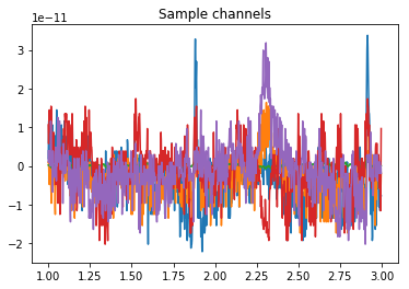
# Extract data from the first 5 channels, from 1 s to 3 s.
sfreq = raw.info['sfreq']
data, times = raw[:5, int(sfreq * 1):int(sfreq * 3)]
_ = plt.plot(times, data.T)
_ = plt.title('Sample channels')

png

Selecting subsets of channels and samples

It is possible to use more intelligent indexing to extract data, using channel names, types or time ranges.

Pull all MEG gradiometer channels: Make sure to use .copy() or it will overwrite the data

meg_only = raw.copy().pick_types(meg=True)
eeg_only = raw.copy().pick_types(meg=False, eeg=True)

The MEG flag in particular lets you specify a string for more specificity

grad_only = raw.copy().pick_types(meg='grad')

Or you can use custom channel names

pick_chans = ['MEG 0112', 'MEG 0111', 'MEG 0122', 'MEG 0123']
specific_chans = raw.copy().pick_channels(pick_chans)
print(meg_only)
print(eeg_only)
print(grad_only)
print(specific_chans)

<Raw  |  sample_audvis_raw.fif, n_channels x n_times : 305 x 166800 (277.7 sec), ~391.7 MB, data loaded>
<Raw  |  sample_audvis_raw.fif, n_channels x n_times : 59 x 166800 (277.7 sec), ~78.2 MB, data loaded>
<Raw  |  sample_audvis_raw.fif, n_channels x n_times : 203 x 166800 (277.7 sec), ~261.7 MB, data loaded>
<Raw  |  sample_audvis_raw.fif, n_channels x n_times : 4 x 166800 (277.7 sec), ~8.1 MB, data loaded>

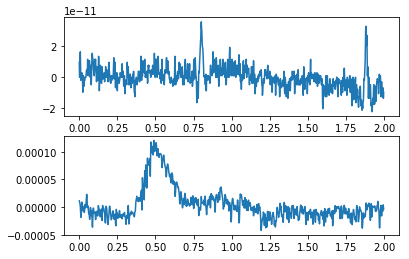
Notice the different scalings of these types

f, (a1, a2) = plt.subplots(2, 1)
eeg, times = eeg_only[0, :int(sfreq * 2)]
meg, times = meg_only[0, :int(sfreq * 2)]
a1.plot(times, meg[0])
a2.plot(times, eeg[0])
del eeg, meg, meg_only, grad_only, eeg_only, data, specific_chans

png

You can restrict the data to a specific time range

raw = raw.crop(0, 50)  # in seconds
print('New time range from', raw.times.min(), 's to', raw.times.max(), 's')

New time range from 0.0 s to 50.00041705299622 s

And drop channels by name

nchan = raw.info['nchan']
raw = raw.drop_channels(['MEG 0241', 'EEG 001'])
print('Number of channels reduced from', nchan, 'to', raw.info['nchan'])

Number of channels reduced from 376 to 374

Concatenating Raw objects

Raw objects can be concatenated in time by using the raw.append function. For this to work, they must have the same number of channels and their Info structures should be compatible.

# Create multiple Raw objects
raw1 = raw.copy().crop(0, 10)
raw2 = raw.copy().crop(10, 20)
raw3 = raw.copy().crop(20, 40)

# Concatenate in time (also works without preloading)
raw1.append([raw2, raw3])
print('Time extends from', raw1.times.min(), 's to', raw1.times.max(), 's')

Time extends from 0.0 s to 40.00399655463821 s

Visualizing Raw data

All of the plotting method names start with plot. If you’re using IPython console, you can just write raw.plot and ask the interpreter for suggestions with a tab key.

To visually inspect your raw data, you can use:

raw.plot(block=True, lowpass=40);

png

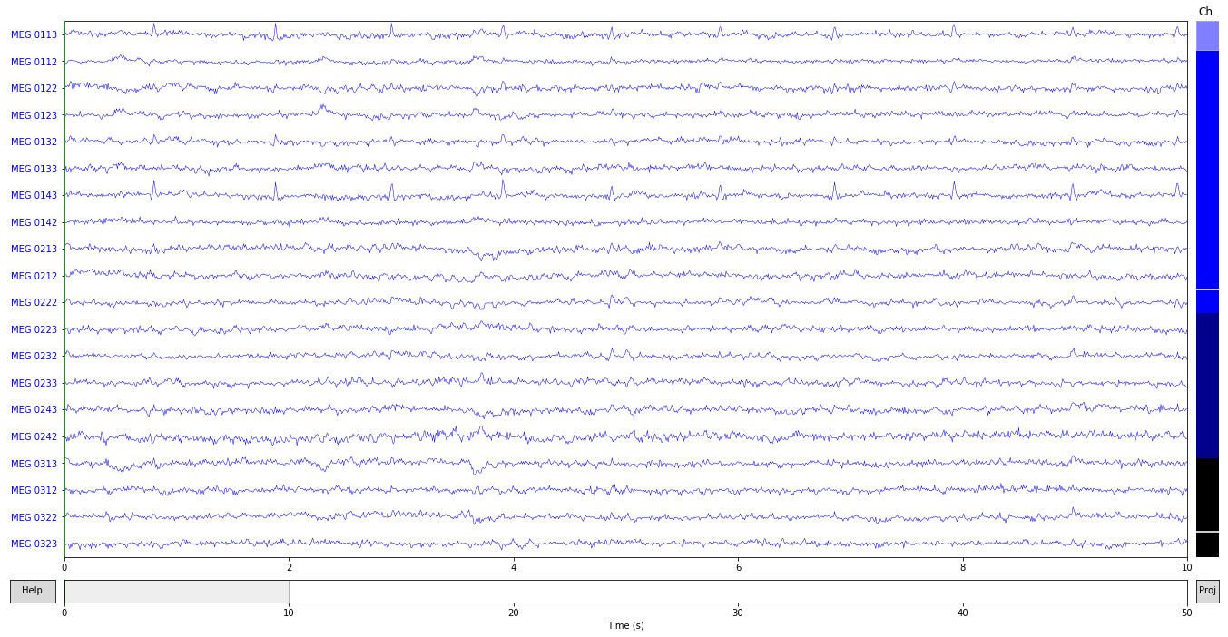
The channels are color coded by channel type.

MEG = blue, EEG = black
Bad channels on scrollbar color coded gray.
Clicking the lines or channel names on the left, to mark or unmark a bad channel interactively.
+/- keys to adjust the scale (also = works for magnifying the data).
Initial scaling factors can be set with parameter scalings.
If you don’t know the scaling factor for channels, you can automatically set them by passing scalings=’auto’.
With pageup/pagedown and home/end keys you can adjust the amount of data viewed at once.

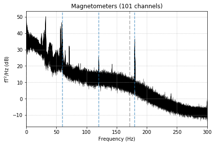
We can also plot the PSD to inspect:

Power line
Bad channels
Head position indicator coils
Whether data is filtered or not

fig, ax = plt.subplots(1, 1)
raw.copy().pick_types(meg='mag').plot_psd(spatial_colors=False, show=False,
                                          ax=ax);
for freq in [60., 120., 180.]:
    ax.axvline(freq, linestyle='--', alpha=0.6)

Effective window size : 3.410 (s)

png

Exercises

1) Quite often the EOG channel is not marked correctly in the raw data. You may need to rename it. Can you figure out how to do this?

# your code here

2) How will you check that at least one EEG channel exists in the data?

# your code here

3) Can you plot the data in the trigger channel?

HINT: The channel type is called ‘stim’

from mne import pick_types
import matplotlib.pyplot as plt

# your code here